Code
library(tidyverse)
library(corrr)
library(formattable)
requireNamespace("bit64")Liang Zhang
June 8, 2022
pivot_wider_indices <- function(data) {
  data |>
    add_count(user_id, game_name) |>
    mutate(
      game_index = if_else(
        n == 1,
        game_name,
        str_c(game_name, index_name, sep = "-")
      )
    ) |>
    pivot_wider(
      id_cols = user_id,
      names_from = game_index,
      values_from = test
    )
}
format_dt <- function(x) {
  x |>
    mutate(across(c(r, abs_r, icc), ~ digits(., 2))) |>
    formattable(
      list(
        abs_r = formatter(
          "span",
          style = ~ style(
            color =
              case_when(
                abs_r > quantile(abs_r, 0.75) ~ "red",
                abs_r > quantile(abs_r, 0.25) ~ "blue",
                TRUE ~ "green"
              )
          )
        ),
        icc = color_tile("transparent", "pink")
      )
    ) |>
    as.datatable(rownames = FALSE)
}targets::tar_load(
reliability_test_retest,
store = here::here("preproc/_targets")
)
ind_filt <- readxl::read_excel(here::here("config/indices_filtering.xlsx"))
indices_clean <- targets::tar_read(
indices_clean,
store = here::here("preproc/_targets")
) |>
inner_join(
filter(ind_filt, check_result %in% c("target", "target-low")) |>
select(game_name, index_name, reversed) |>
add_row(
game_name = "瑞文高级推理",
index_name = "nc_test",
reversed = FALSE
),
by = c("game_name", "index_name")
) |>
mutate(test = if_else(reversed, -test, test))A basic principle choosing tasks for measuring training transfer effect is based on the correlations between the chosen tasks and the target tasks. Two types of target tasks are now selected:
Here the correlations with these two types of tasks are calculated as follows.
indices_clean |>
  filter(game_name_abbr != "RAPM") |>
  inner_join(
    indices_clean |>
      filter(
        game_name_abbr == "RAPM",
        index_name == "nc_test"
      ) |>
      select(user_id, rapm = test),
    by = "user_id"
  ) |>
  group_by(game_name, index_name) |>
  summarise(
    n = sum(!is.na(test) & !is.na(rapm)),
    r = cor(test, rapm, use = "complete"),
    .groups = "drop"
  ) |>
  mutate(abs_r = abs(r)) |>
  arrange(desc(abs_r)) |>
  left_join(
    reliability_test_retest |>
      select(game_name, index_name, icc = icc_no_outlier),
    by = c("game_name", "index_name")
  ) |>
format_dt()indices_clean |>
filter(game_name_abbr != "NVR") |>
inner_join(
indices_clean |>
filter(game_name_abbr == "NVR") |>
select(user_id, nvr = test),
by = "user_id"
) |>
group_by(game_name, index_name) |>
summarise(
n = sum(!is.na(test) & !is.na(nvr)),
r = cor(test, nvr, use = "complete"),
.groups = "drop"
) |>
filter(n > 100) |>
mutate(abs_r = abs(r)) |>
arrange(desc(abs_r)) |>
left_join(
reliability_test_retest |>
select(game_name, index_name, icc = icc_no_outlier),
by = c("game_name", "index_name")
) |>
format_dt()mean_scores <- indices_clean |>
filter(
game_name_abbr == "NVR" |
(game_name_abbr == "RAPM" & index_name == "nc_test")
) |>
pivot_wider(
id_cols = user_id,
names_from = game_name_abbr,
values_from = test
) |>
mutate(
across(c(NVR, RAPM), ~ scale(.)[, 1]),
score_avg = map2_dbl(NVR, RAPM, ~ (.x + .y) / 2)
)
indices_clean |>
filter(!game_name_abbr %in% c("NVR", "RAPM")) |>
inner_join(mean_scores, by = "user_id") |>
group_by(game_name, index_name) |>
summarise(
n = sum(!is.na(test) & !is.na(score_avg)),
r = cor(test, score_avg, use = "complete"),
.groups = "drop"
) |>
filter(n > 100) |>
mutate(abs_r = abs(r)) |>
arrange(desc(abs_r)) |>
left_join(
reliability_test_retest |>
select(game_name, index_name, icc = icc_no_outlier),
by = c("game_name", "index_name")
) |>
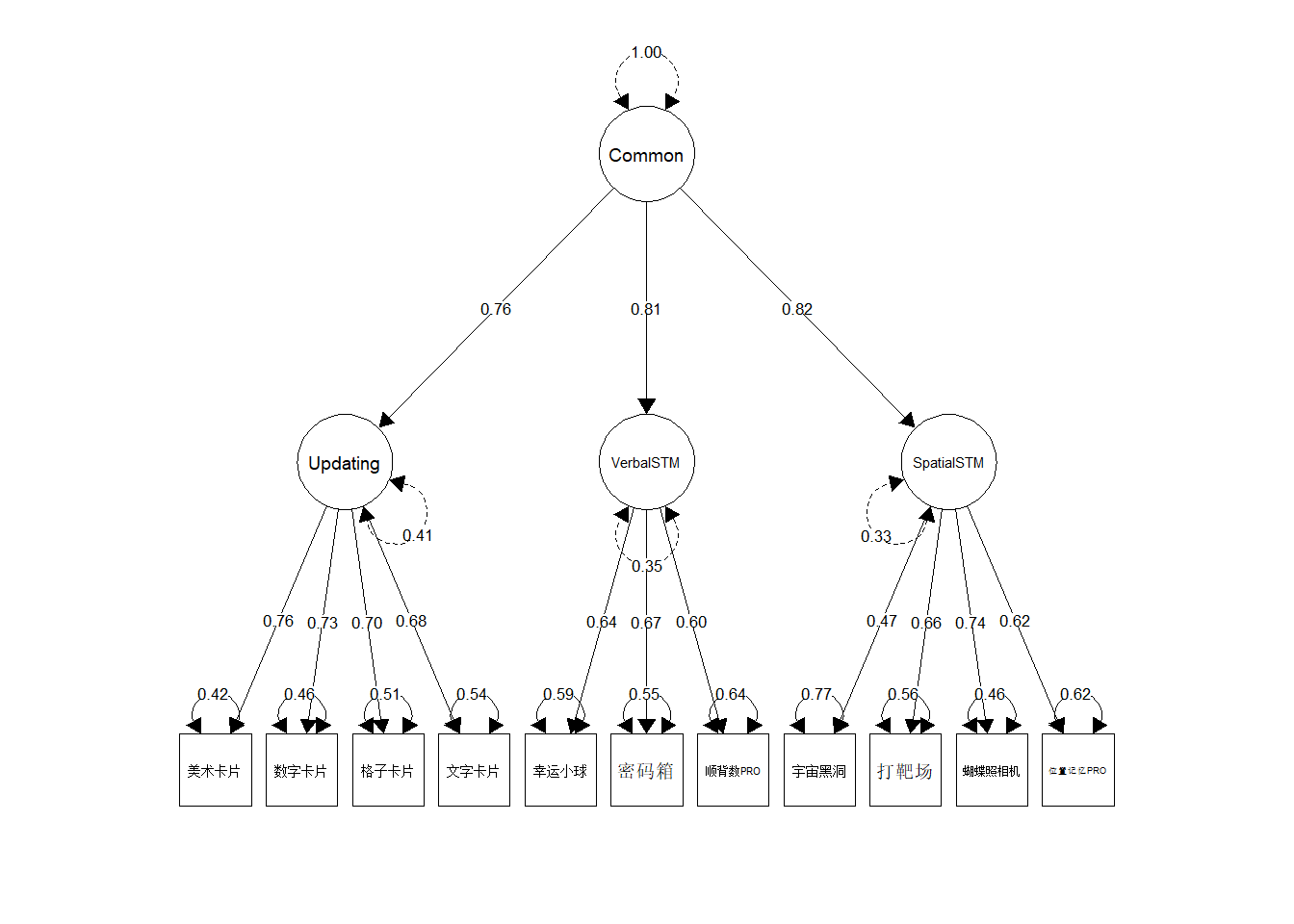
format_dt()fitted <- lavaan::cfa(
'Common =~ Updating + VerbalSTM + SpatialSTM
Updating =~ `美术卡片` + `数字卡片` + `格子卡片` + `文字卡片`
VerbalSTM =~ `幸运小球` + `密码箱` + `顺背数PRO`
SpatialSTM =~ `宇宙黑洞` + `打靶场` + `蝴蝶照相机` + `位置记忆PRO`',
indices_viswm, std.lv = TRUE, std.ov = TRUE,
estimator = "MLR", missing = "ml"
)
semPlot::semPaths(
fitted, what = "std", edge.color = "black", layout = "tree2",
sizeMan = 6, sizeLat = 8, edge.label.cex = 0.6, intercepts = FALSE,
nCharEdges = 5, esize = 1, trans = 1, nCharNodes = 0,
bifactor = "Common"
)
lavaan 0.6-11 ended normally after 34 iterations

  Estimator                                         ML
  Optimization method                           NLMINB
  Number of model parameters                        36

  Number of observations                           515
  Number of missing patterns                        26

Model Test User Model:
                                               Standard      Robust
  Test Statistic                                119.832     114.108
  Degrees of freedom                                 41          41
  P-value (Chi-square)                            0.000       0.000
  Scaling correction factor                                   1.050
       Yuan-Bentler correction (Mplus variant)

Model Test Baseline Model:

  Test statistic                              1493.661    1199.093
  Degrees of freedom                                55          55
  P-value                                        0.000       0.000
  Scaling correction factor                                  1.246

User Model versus Baseline Model:

  Comparative Fit Index (CFI)                    0.945       0.936
  Tucker-Lewis Index (TLI)                       0.926       0.914

  Robust Comparative Fit Index (CFI)                         0.946
  Robust Tucker-Lewis Index (TLI)                            0.928

Loglikelihood and Information Criteria:

  Loglikelihood user model (H0)              -6490.246   -6490.246
  Scaling correction factor                                  1.867
      for the MLR correction
  Loglikelihood unrestricted model (H1)      -6430.330   -6430.330
  Scaling correction factor                                  1.432
      for the MLR correction

  Akaike (AIC)                               13052.493   13052.493
  Bayesian (BIC)                             13205.283   13205.283
  Sample-size adjusted Bayesian (BIC)        13091.013   13091.013

Root Mean Square Error of Approximation:

  RMSEA                                          0.061       0.059
  90 Percent confidence interval - lower         0.049       0.046
  90 Percent confidence interval - upper         0.074       0.071
  P-value RMSEA <= 0.05                          0.071       0.116

  Robust RMSEA                                               0.060
  90 Percent confidence interval - lower                     0.047
  90 Percent confidence interval - upper                     0.074

Standardized Root Mean Square Residual:

SRMR 0.038 0.038scores_latent <- bind_cols(
select(indices_viswm, user_id),
lavaan::predict(fitted) |>
unclass() |>
as_tibble()
)
indices_clean |>
inner_join(
scores_latent,
by = "user_id"
) |>
group_by(game_name, index_name) |>
summarise(
n = sum(!is.na(test) & !is.na(Common)),
r = cor(test, Common, use = "complete"),
.groups = "drop"
) |>
mutate(abs_r = abs(r)) |>
arrange(desc(abs_r)) |>
left_join(
reliability_test_retest |>
select(game_name, index_name, icc = icc_no_outlier),
by = c("game_name", "index_name")
) |>
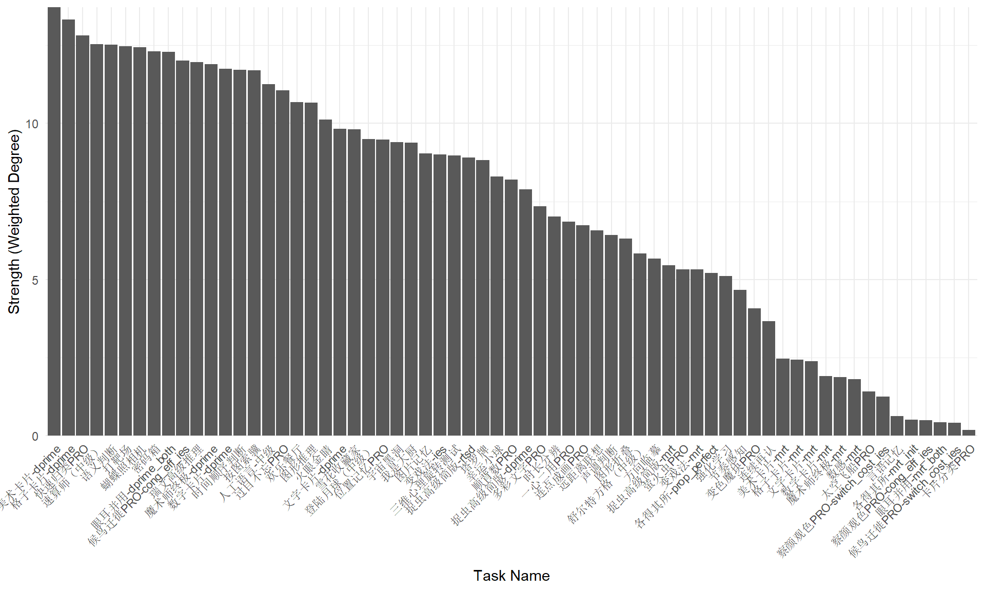
format_dt()Another task is to find the core tasks for the cognition. A direct method is to find the task that has the largest sum of correlations with all other tasks. It is so-called strength of nodes in network.
library(tidygraph)
graph <- indices_clean |>
  pivot_wider_indices() |>
  select(-user_id) |>
  correlate() |>
  stretch(na.rm = TRUE, remove.dups = TRUE) |>
  filter(r > 0.15) |>
  tidygraph::as_tbl_graph(directed = FALSE)
strengths <- graph |>
  activate(nodes) |>
  mutate(strength = centrality_degree(weights = r)) |>
  as_tibble() |>
  arrange(desc(strength))
strengths |>
  mutate(strength = digits(strength, 1)) |>
  formattable(
    list(strength = color_text("green", "red"))
  ) |>
  as.datatable()